Search
Feeds
Archives
About
Links
BLOG
Sunday 28 July 2019 at 09:06 am.This section presents some examples of the command line capabilities of TerraceM outside the Graphic user interface.
Loading TerraceM-2 Maptools outputs
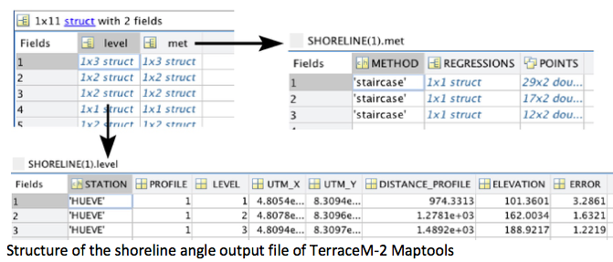
TerraceM-2 Maptools creates several Matlab® files used for data exchange between the other TerraceM-2 modules. These files can be called independently to create customized plots. In this example, we load the main output files containing the shoreline angles and swath profiles.
%Load swath profiles
load('HUEVE_swath.mat');
%Load shoreline angles
load('HUEVE_SHORELINES.mat');
The shoreline-angle file (.mat) is a structure containing several fields that define: a) method (met) used to map the shoreline angles, including the linear regression coefficients and points used for mapping, and b) the shoreline angle level (level), which includes the profile, elevation, error, map coordinates, location along profile and the station or mapping site name.
Displaying swath profiles and shorelines angles mapped in TerraceM-2
This excercise follows the previous example.
Here we present an example plotting swath profiles and shoreline angles using the output files of TerraceM-2 Maptools.
i=2; %profile number
j=1; %marine terrace level
%these values can be eventually looped to plot all mapped shoreline angles
 %extract the linear regressions for platform and cliff
cliff=SHORELINE(i).met(j).REGRESSIONS.cliff;
plat=SHORELINE(i).met(j).REGRESSIONS.plat;
points=SHORELINE(i).met(j).POINTS;
%extract the shoreline angle
SH(1)=SHORELINE(i).level(j).DISTANCE_PROFILE;
SH(2)=SHORELINE(i).level(j).ELEVATION;
SH(3)=SHORELINE(i).level(j).ERROR;
 %plot the result
figure
hold on; plot(swath(i).x,swath(i).z_max,'-k',swath(i).x,swath(i).z_min,...
    '-k',swath(i).x,swath(i).z_mean,'-k');%plot the swath profile
plot(cliff(:,1),cliff(:,2),'--r'); plot(cliff(:,1),cliff(:,4),'--r');%cliff points
plot(cliff(:,1),cliff(:,3),'-r');plot(plat(:,1),plat(:,2),'--r');%platform points
plot(plat(:,1),plat(:,4),'--r');plot(plat(:,1),plat(:,3),'-r');%regressions
errorbar(SH(1),SH(2),SH(3),'ok'); plot(SH(1),SH(2),'ok',...  %shoreline angle
    'MarkerFaceColor','r','Markersize',6);
xlabel('Distance along profile (m)');ylabel('Elevation (m)');%axis labels
Creating swath profiles from shapefile polygons outside the GUI environment
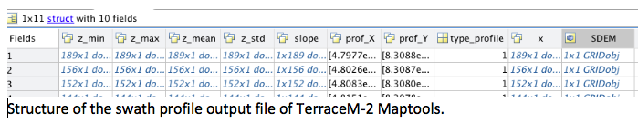
Swath profiles can be generated using the TerraceM_makeswath.m function and Topotoolbox. The inputs are a DEM in geotiff (.tif) or Esri grid format (.asc) and a shapefile containing the swath profiles boxes, which may be created using the rectangle tool. The output is a structure containing the distance, minimum, mean, maximum and slope of a swath profile.
%Add path to topotoolbox folder, TerraceM-2 Maptools, and dem and shapefile.
addpath /Users/TerraceM_2018/Stations/HUEVO
addpath /Users/TerraceM_2018/topotoolbox-master
addpath /Users/TerraceM_2018/TerraceM_Maptools
Box=shaperead('Huevo_clip.shp'); %Shapefile containing the profiles boxes
DEM=GRIDobj('DEM_huevo.tif'); %DEM generated using Topotoolbox
profnum=2; %Profile number to process
%Create swath function
swat=TerraceM_makeswath(DEM,Box,profnum);
%Display swath profile
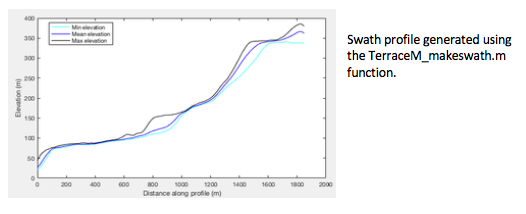
figure
plot(swat.x,swat.z_min,'-c',swat.x,swat.z_mean,'-b',swat.x,swat.z_max,'-k');%plot the swath lines
xlabel('Distance along profile (m)'); ylabel('Elevation (m)');
legend('Min elevation','Mean elevation','Max elevation')
Mapping shoreline angles outside the GUI environment
This excercise follows the swath profile plot excercise presented before.
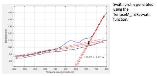
We can directly map shoreline angles calling the function TerraceM_staircase.m, which displays an interactive window to map the shoreline angle by selecting the paleo-platform and paleo-cliff. Outputs include the shoreline angle elevation and its associated error (shoreline), the points used to fit the linear regressions (points), and the linear regression coefficients and 95% confidence bounds (regr).
%Mapping a single shoreline angle
[shoreline,points,regr]=TerraceM_staircase(swat);
TerraceM-2 LEM scripts
The TerraceM-2 LEM module includes two functions that can be used to create custom models, export results in video formats, and compare the results to swath profile topography.
Creating a LEM movie
Two options exist to create a LEM movie: Simple or customized display. The optional input parameters allow for custom movie size, style, and speed.
clear
%add path to TerraceM-2 LEM and the sealevel folders
addpath /Users/TerraceM_2018/TerraceM_LEM
addpath /Users//TerraceM_2018/TerraceM_LEM/sealevel
%inputs
sl=load('Bintanja_total.mat');%load a sea-level curve
%parameters in structure format
param.tmax=500;%max time (ka)
param.tmin=0;%min time (ka)
param.dt=100;%bin size of time intervals (yrs)
param.dx=5;%bin size of x axis (m)
param.sill=150;%m, avoid sill by adding an extremely deep value
param.slope_shelf=10;%initial slope model (deg)
param.uplift_rate=1.8; %m/ka
param.initial_erosion=0.3;% initial erosion rate or E0 (m/yr)
param.cliff_diffusion=0.02;% cliff slope difussion (m^2/yr)
param.wave_height=5;%wave height (m)
param.vxx=0;%manually extend x axis if model run out of bounds
param.smth=40;%smooth factor of sea-level curve (yr)
param.video=1;%video mode activated
%optional input parameters, ignore for quick video display
param.cumula=0;%cummulative plot deactivated
param.snap=90;%number of video frames
%create axes for video
param.h1=subplot(3,1,1:2); param.h2=subplot(3,1,3);
%call LEM function
[LEM]=TerraceM_anderson(sl,param);
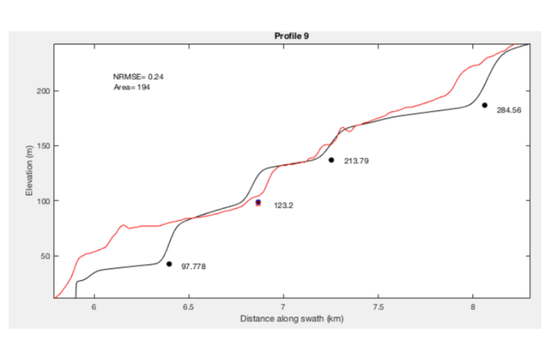
Comparing measured and synthetic LEM terraces
The topographic expression of marine terraces can be directly compared to LEM results by tying them using a single shoreline angle. This requires assigning an estimated or measured age to the shoreline angle and adjusting the input parameters to minimize the weighted root mean squared error WRMSE or the difference between model and observations. To compare modeled and measured topography, we use the TerraceM_rms_fit.m function and a swath profile .mat input file, and select a piercing point shoreline angle. The function uses two LEM’s, one including all the user-defined parameters and the second with slope diffusion equal to 0, in order to find the position of shoreline angles in the LEM. Here we present an example fitting a profile with a constant uplift rate (Fig 5SP); note that the quality of the fit decreases upwards suggesting that this area was probably affected by variable uplift rate along time.
clear
%addpath to TerraceM-2 LEM folders and input files
addpath /Users/TerraceM_2018/TerraceM_LEM
addpath /Users/TerraceM_2018/TerraceM_LEM/sealevel addpath /Users/TerraceM_2018/Stations/HUEVO/HUEVE
%First load a profile and the shoreline angle
load('HUEVE_swath.mat') %loadswath profiles
load('HUEVE_SHORELINES.mat') %load shoreline angles
i=9; %profile number
j=1; %marine terrace level
%extract the shoreline angle
SH(1)=SHORELINE(i).level(j).DISTANCE_PROFILE; SH(2)=SHORELINE(i).level(j).ELEVATION; SH(3)=SHORELINE(i).level(j).ERROR;

%extract the swath profile
SW(:,1)=swath(i).x;
SW(:,2)=swath(i).z_min;
SW(:,3)=swath(i).z_mean;
SW(:,4)=swath(i).z_max;
%create LEM’s
%LEM input parameters in structure format
sl=load('Bintanja_total.mat');%load a sea-level curve

param.tmax=500;%max time (ka)

param.tmin=0;%min time (ka)

param.dt=100;%bin size of time intervals (yrs)

param.dx=5;%bin size of x axis (m)

param.sill=150;%avoid sill effect of sl by adding an extremely deep value (m)
param.slope_shelf=4;%initial slope model (deg)

param.uplift_rate=0.8; %uplift rate m/ka

param.initial_erosion=0.05;% initial erosion rate or E0 (m/yr)
param.cliff_diffusion=0.005;% cliff slope diffusion (m^2/yr)
param.wave_height=5;%wave height (m)

param.vxx=0;%manually extend x axis if model run out of bounds (m)
param.smth=40;%smooth factor of sea-level curve (yr)

param.video=0;%video mode deactivated
param2=param; %modify diffusion to cero for the default LEM
param2.cliff_diffusion=0;% cliff slope diffusion for the default model (m^2/yr)
%Create a LEM
[LEM]=TerraceM_anderson(sl,param);
%Create default LEM without slope diffusion to locate the shoreline angles
[LEM2]=TerraceM_anderson(sl,param2);
%LEM fitting parameters

age=125;%estimated shoreline angle age (ka)

ratio=100;%search ratio to avoid overlapping shoreline angles in LEM (yr)
cycle=15000;%mean span between glacial cycles (yr), smaller value increase detail in shoreline angle detection
%profile subset for fitting

up=9;%distance inlands from shoreline angle (km)
down=3;%distance seawards from shoreline angle (km)
mode=1;%plot fit activated
savepdf=0;%save figure deactivated
%%%% run the fit function
[Result,MOD]=TerraceM_rms_fit(LEM,LEM2,i,SW,SH,age,ratio,cycle,up,down,mode,savepdf);
TerraceM-2 DIM scripts
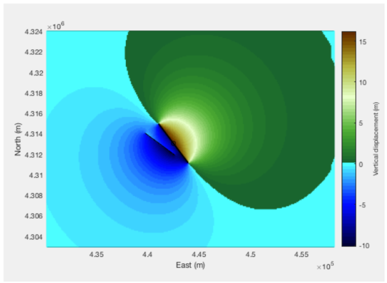
Creating a custom elastic dislocation model using mapped faults in a polyline shapefile as input
Elastic dislocation models can be developed using inputs as Shapefiles and the function TerraceM_okada.m; here we present an example using two faults.
clear
%set directories to TerraceM-2 okada functions and input files
addpath /Users/TerraceM_2018/stations/San_Andreas/SANDREAS/SANDREAS_EXPORT
addpath /Users/TerraceM_2018/TerraceM_DIM
%Input shapefiles created in arcgis
%faults, a polyline shapefile containing the faults
Sf=shaperead('SANDREAS_fault.shp');% faults polyline file, contains 2 faults
%box is a polygon shapefile of the area for modeling, usually is a square
%and should be bigger than the fault extent
Bx=shaperead('Sandreas_box.shp');
%Input parameters in structure format
param.d=100;%cellsize (m)
param.Dip(1)=80;%dip of fault 1 (deg)
param.Dip(2)=80;%dip of fault 2 (deg)
param.Slip(1)=5;%Slip fo fault 1 (m or m/ka)
param.Slip(2)=25;%Slip fo fault 2 (m or m/ka)
param.Updip(1)=0;%Updip of fault 1 (m)
param.Updip(2)=0;%Updip of fault 2 (m)
param.Downdip(1)=10000;%Downdip of fault 1 (m)
param.Downdip(2)=10000;%Downdip of fault 2 (m)
param.Rake(1)=90;%Rake of fault 1 (deg)
param.Rake(2)=90;%Rake of fault 2 (deg)
param.pplot=1;%plot result activated
%call the function to create dislocation models
[E3,N3,El,Nl,U]=TerraceM_okada(Sf,Bx,param);
TerraceM ICESat-2
This section include several python scripts to create a query, submit it, check the server status and download ICESat-2 data. ICESat-2 satellite mission was lauched in 2018, it provides high resolution 2D topographic profiles based on laser rebound similar as LiDAR. This data can be filtered by vegetation allowing obtaining bare-earth high-resolution topographic profiles (20-cm point spacing). TerraceM ICESat-2 include a GUI but also several functions to download and process t5his data, here we show a step by step usage of these python functions:
1) Create a query:
Queries allow identify available data for a set of parameters. We uyse the script TEST_query.py, this script communicates with the HARMONY server of NASA and return the the total number of granules (track covering the area) and the collection ID (Name of the data group for download). The collection ID is specially important for the next steps including submit job and test status:
# Test_query.py
from icesat2_query import icesat2_query
# --------------------------
# Query CMR ICESAT-2 database of whole granules
# --------------------------
########## INPUTS ##################################
bbox = [-75.23, -15.47, -75.03, -15.33]
dates = ("2023-01-01", "2023-01-31")
product = "ATL03"   # ICESat-2 product you can also set here ATL08 or ATL06
version = "006"     # Version of the product

####################################################
collection_id, info, resp = icesat2_query(product, bbox, dates, version)
print(f"\nFound {info['total_granules']} granules – DONE!")
print(f"Collection ID: {collection_id}")
# --------------------------
# Save only the collection ID to a text file
# --------------------------
with open("collection_id.txt", "w") as f:

f.write(collection_id)
2) Submit Job:
If you are satisfied with the number of granules provided by the query you can proceed to submit the job for download. For this we use the script Test_submit_job.py. This script uses your Earthdata credentials and the collection ID amongh others. Importantly after submitting a job you will obtain a JOB ID that is an identifier of the job you submitted, ithis identifier is important either to test the job status and to finally download the data.
# Test_submit_job.py
import subprocess
# --------------------------
# Call Harmony job script
# --------------------------
########## INPUTS #################################v#
username = "yourusername"
password = "yourpassword"
bbox = [-75.23, -15.47, -75.03, -15.33]
dates = ("2023-01-01", "2023-01-31")
collection_id = "C2596864127-NSIDC_CPRD"
output_dir = "./ICESat2_jobs" # folder to save the files
##########################################################
cmd = [
"python",
"PY_MAT_Send_Job.py",
"--collection_id", collection_id,
"--west", str(bbox[0]),
"--south", str(bbox[1]),
"--east", str(bbox[2]),
"--north", str(bbox[3]),
"--start_year", dates[0][0:4],
"--start_month", dates[0][5:7],
"--start_day", dates[0][8:10],
"--end_year", dates[1][0:4],
"--end_month", dates[1][5:7],
"--end_day", dates[1][8:10],
"--username", username,
"--password", password,
"--output_dir", output_dir
]
print("\nRunning Harmony job…")
subprocess.run(cmd)
3) Check job status:
After the job is sumbitted the Harmony severs need to subset the data according your requirements, this can take some time depending of the amount of data, ranging from minutes to a couple of hours. I never waited more than one hour, even downloading more than 50 gb of data. To check the status of your job we use the Test_status.py script, this script make a simple call to HARMONY and return the job status. When the status is ready, you can proceed to download the data.
# Test_status.py
import subprocess
# -----------------------------
# User parameters
# -----------------------------
########### INPUTS #######################################################
username = "yourusername"
password = "yourpassword"
job_id   = "92c582e3-48d8-4d78-b359-caef389c633f"  # replace with actual Job ID
#############################################################################
# Path to the status script
status_script = "PY_MAT_Status_Job.py"
# -----------------------------
# Build command
# -----------------------------
cmd = [
    "python", status_script,
    "--username", username,
    "--password", password,
    "--job_id", job_id
]
# -----------------------------
# Run the script and capture output
# -----------------------------
print("Checking Harmony job status…\n")
subprocess.run(cmd)
4) Downloading the ICESat-2 data:
Finally when the status is ready you can proceed to download the data. For this we use the TEST_download_data.py script. In this script you need again your credentials, your job ID and also you can define a download folder. This process can take some time depending of your internet speed.
# Test_download_data.py
import subprocess
# -----------------------------
# User parameters
# -----------------------------
########### INPUTS #######################################################
username = "yourusername"
password = "yourpassword"
job_id     = "92c582e3-48d8-4d78-b359-caef389c633f"
output_dir = "./ICESat2_jobs"  # folder to save the files
#########################################################################
# Path to the download script
download_script = "PY_MAT_Download_Job.py"
# -----------------------------
# Build command
# -----------------------------
cmd = [
    "python",
    download_script,
    "--username", username,
    "--password", password,
    "--job_id", job_id,
    "--output_dir", output_dir
]
# -----------------------------
# Run the download script
# -----------------------------
print("Starting download of Harmony job results…\n")
subprocess.run(cmd)
5) Converting data format:
Finally when all the data is download we need to make is readable by other software such as matlab. The downloaded data is in .h5 format in its latest version. Sadly Matlab works with older .h5 format releases, but we can easily conver the /h5 files to the old format. This process is fas and ensure compatibility so you can load it in matlab and continue processing. For this we use the TEST_convert_H5.py, this script requeres you to indicate the folder containing the original .h5 files and the output folder for the reformated files.
#TEST_convert_H5.py
import subprocess
import os
# -----------------------------
# User parameters
# -----------------------------
########### INPUTS ############################################
input_dir  = "./ICESat2_jobs"       # Folder with HDF5 files to convert
output_dir = "./ICESat2_converted"       # Folder to save converted files
##################################################################
# Path to the conversion script
convert_script = "convert_h5_to_oldformat.py"
# Check if script exists
if not os.path.isfile(convert_script):
    raise FileNotFoundError(f"Conversion script not found: {convert_script}")
# -----------------------------
# Build command
# -----------------------------
cmd = [
    "python",
    convert_script,
    "--input_dir", input_dir,
    "--output_dir", output_dir
]
# -----------------------------
# Run the conversion script
# -----------------------------
print("Starting HDF5 conversion…\n")
subprocess.run(cmd)
